以波士顿房价预测为例介绍机器学习中的线性回归。
线性回归(Linear Regression)
参考:
Machine Learning小结(1):线性回归、逻辑回归和神经网络
环境:
操作系统:Ubuntu 18.04
编程语言:Python 3.6.7
第三方库:numpy\matplotlib\scikit-learn
1 | |
定义
给定数据集D={(x1, y1), (x2, y2), … },我们试图从此数据集中学习得到一个线性模型,这个模型尽可能准确地反应x(i)和y(i)的对应关系。这里的线性模型,就是属性(x)的线性组合的函数,可表示为:
\[f(x) = w_1x_1 + w_2x_2 + ... + w_nx_n + b\]向量表示为:
\[f(x) = W^TX + b\]其中,W是由(w1, w2, …, wn)组成的列向量,表示weight,即权重,b表示bias,即偏差。
在机器学习中,我们希望可以建立一个函数,使其尽可能符合现有的数据分布,这样我们就可以通过这个函数对未知的数据进行预测。线性回归需要解决的问题就是如何求得参数W和b,使函数获得最优解,即使其预测结果更接近真实值。
数据处理
首先我们需要获取数据集,然后根据数据集的分布确定我们的预测函数。
采用sklearn的波士顿房价数据集:
1 | |
波士顿房价数据集中data一共包含13个特征,target是最后的房价。通过以下代码可以查看其各项属性:
1 | |
.. _boston_dataset:

Boston house prices dataset
---------------------------

**Data Set Characteristics:**

 :Number of Instances: 506

 :Number of Attributes: 13 numeric/categorical predictive. Median Value (attribute 14) is usually the target.

 :Attribute Information (in order):
        - CRIM     per capita crime rate by town
        - ZN       proportion of residential land zoned for lots over 25,000 sq.ft.
        - INDUS    proportion of non-retail business acres per town
        - CHAS     Charles River dummy variable (= 1 if tract bounds river; 0 otherwise)
        - NOX      nitric oxides concentration (parts per 10 million)
        - RM       average number of rooms per dwelling
        - AGE      proportion of owner-occupied units built prior to 1940
        - DIS      weighted distances to five Boston employment centres
        - RAD      index of accessibility to radial highways
        - TAX      full-value property-tax rate per $10,000
        - PTRATIO  pupil-teacher ratio by town
        - B        1000(Bk - 0.63)^2 where Bk is the proportion of blacks by town
        - LSTAT    % lower status of the population
        - MEDV     Median value of owner-occupied homes in $1000's

 :Missing Attribute Values: None

 :Creator: Harrison, D. and Rubinfeld, D.L.

This is a copy of UCI ML housing dataset.
https://archive.ics.uci.edu/ml/machine-learning-databases/housing/


This dataset was taken from the StatLib library which is maintained at Carnegie Mellon University.

The Boston house-price data of Harrison, D. and Rubinfeld, D.L. 'Hedonic
prices and the demand for clean air', J. Environ. Economics & Management,
vol.5, 81-102, 1978.   Used in Belsley, Kuh & Welsch, 'Regression diagnostics
...', Wiley, 1980.   N.B. Various transformations are used in the table on
pages 244-261 of the latter.

The Boston house-price data has been used in many machine learning papers that address regression
problems.

.. topic:: References

   - Belsley, Kuh & Welsch, 'Regression diagnostics: Identifying Influential Data and Sources of Collinearity', Wiley, 1980. 244-261.
   - Quinlan,R. (1993). Combining Instance-Based and Model-Based Learning. In Proceedings on the Tenth International Conference of Machine Learning, 236-243, University of Massachusetts, Amherst. Morgan Kaufmann.
为了便于测试模型的准确性,训练出准确性最好,泛化程度最高的模型,我们需要将模型分割成训练集、验证集和测试集。方便起见,在此我们仅将其分为训练集和测试集。使用sklearn的split工具分割数据:
1 | |
train_test_split将数据集随机分为了训练集和测试集两部分,分别占原数据集的95%和5%。后面将使用这两个数据集训练模型并对其进行检测。
选择数据集中第6个特征作为自变量,target作为因变量。根据上面的属性可以看出,该特征为average number of rooms per dwelling,即住所平均房间数。
1 | |
前向传播
调用matplotlib对所选数据进行绘图:
1 | |
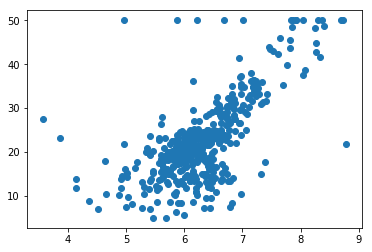
可以看出,数据近似为一个一次函数。因此我们使用以下函数预测数据: \(h(x) = wx + b\) 如果数据分布近似二次函数或其他类型函数,就需要改变预测函数的形式,使其符合数据分布规律。此函数中,h(x)即为该函数预测的房价,x为房间数,w和b是该函数的参数。采用随机值为w和b赋值,可产生第一个预测的函数:
1 | |
x,w和b都是矩阵格式的数据。b和h的维度不一致但也可以进行运算,这是使用了numpy中的广播机制。h即为使用w和b作为参数预测的房价。对其进行绘图:
1 | |
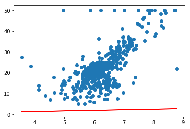
可以看出,此时预测的函数偏差还很大,不能作为最后的结果。
反向传播
反向传播过程需要通过数据集中的target来优化现在的预测函数,使它的预测值尽可能接近真实值。
定义每一个样本的预测结果与真实值之间的偏差的表达式为损失函数(Loss Function),所有损失函数的和为代价函数(Cost Function)。当Cost Function接近最小值,我们就可以认为函数预测的结果已经接近真实值。在线性回归中,使用最小二乘法来定义其损失函数:
\[Loss = [h(x^i) - y^i]^2\]Cost Function是所有Loss的和:
\[J = \frac{1}{2m}\sum\limits_{i = 1}^{m} Loss = \frac{1}{2m}\sum\limits_{i = 1}^{m} [h(x^i) - y^i]^2\]式中m是样本数量。当J接近0的时候,h(x) 近似等于 y,可以认为该函数的预测值接近真实值。1/2m的作用是简化后面的求导运算。
1 | |
完成以上定义以后,我们就可以通过优化w和b来使J接近0,即可获得最佳的预测函数。
梯度下降(Gradient Descent)
结合预测函数h和代价函数J,我们可以得到以下表达式:
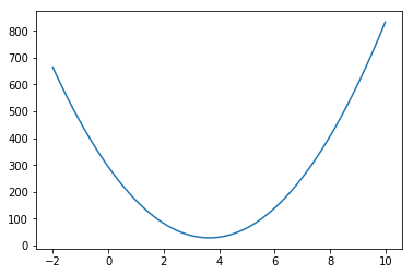
\[J = \frac{1}{2m}\sum\limits_{i = 1}^{m} [h(x^i) - y^i]^2 = \frac{1}{2m}\sum\limits_{i = 1}^{m} [wx^i + b - y^i]^2\]先简化上式,假设b = 0,则该表达式就变成了:
\[J = \frac{1}{2m}\sum\limits_{i = 1}^{m} [wx^i - y^i]^2\]可以看出,现在J的大小只受w的影响。设w为自变量J为因变量,可画出以下图像:
1 | |
任取一个w作为预测函数的初始参数,该参数对应着图像上的一个点。在该点用J对w求导,得到的结果就是梯度,从他的几何意义上来说,就是函数增长的方向。因此,要想使该点到达函数的局部/全局最优点,就需要让w减去这个梯度,使该点沿着函数值减小的方向前进。这就是梯度下降。公式为:
repeat until convergence {
\[\theta := \theta - \alpha\frac{\partial}{\partial \theta}{J(\theta)}\]}
其中,θ是参数,对应预测函数中的w(和b),α是学习率。这个公式的含义就是让θ每次沿梯度下降的方向前进一点,直到函数收敛为止。学习率决定了每次前进的步长,如果学习率太小,训练过程会很慢;如果学习率过大,可能会使参数直接跨过最小值点,导致最后的结果无法收敛。另外,由于随着CostFunction趋近于最小值,函数的梯度逐渐减小,θ前进的步长也会逐渐减小,所以不需要随着训练过程改变α的值。
由于线性回归的CostFunction没有局部最优解,所以梯度下降的结果一定是全局最优解。
最小二乘法的代价函数的导数可以化简为如下形式:
\[\frac{\partial}{\partial w}{J(w)} = \frac{1}{m}\sum\limits_{i = 1}^{m}\{[h(x^i) - y^i]x^i\}\] \[\frac{\partial}{\partial b}{J(b)} = \frac{1}{m}\sum\limits_{i = 1}^{m}[h(x^i) - y^i]\]所以梯度下降的过程为:
repeat until convergence {
\[w := w - \alpha\frac{1}{m}\sum\limits_{i = 1}^{m}\{[h(x^i) - y^i]x^i\}\] \[b := b - \alpha\frac{1}{m}\sum\limits_{i = 1}^{m}[h(x^i) - y^i]\]}*
由于更新参数会导致h发生变化,从而影响后面参数的更新过程,所以需要先完成计算然后同步更新所有参数。
1 | |
使用参数更新前后CostFunction的差值作为判断函数收敛的标志,当差值小于0.00001以后,可以认为函数的梯度为近似为0,函数收敛。
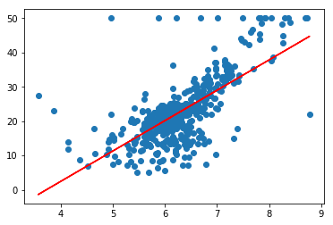
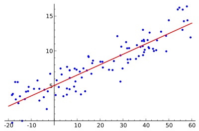
经过训练以后,预测函数已经有了比较好的效果,基本符合实际数据。
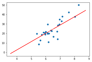
同时,在测试集上,该预测函数同样也基本符合数据分布。